Visualising arc-minutes and arc-seconds

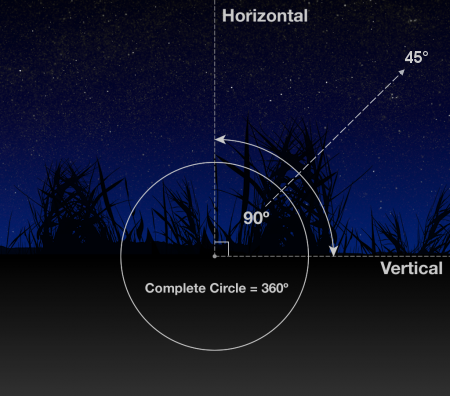
For the purposes of astronomical observation, the apparent size of celestial objects is normally expressed using angular degrees. This begins to make sense when you consider the sky as the inside surface of a sphere, with you as the observer at the centre. Each degree is divided into 60 "minutes", referred to as arc-minutes or minutes of arc. Each arc-minute can in turn be divided into 60 arc-seconds.

In astrophotography, arc-seconds are the most commonly used for a variety of reasons relating to their scale. Because of distortion caused by atmospheric turbulence or "seeing", resolutions higher than around one arc-second are of limited practical use. Due to this, the size of features visible in celestial objects is usually described in arc-seconds, as finer details than this usually can't be resolved. This is why the resolution of telescopes is typically measured in arc-seconds, and pixel scale, which is an important aspect of an imaging setup which will be explored in more detail a bit later, is measured in arc-seconds per pixel.

The fundamental limits on optical observation due to seeing are an issue almost everywhere, but there is some local variation. This is the main reason professional telescopes are typically sited high up on mountaintops, in locations that enjoy some of the most stable air (and reliably clear skies) on earth. It also helps that at a higher altitude, there is simply less atmosphere to look through. Famed planetary astrophotographer Damian Peach favours the Bahamas as an imaging site for similar reasons.

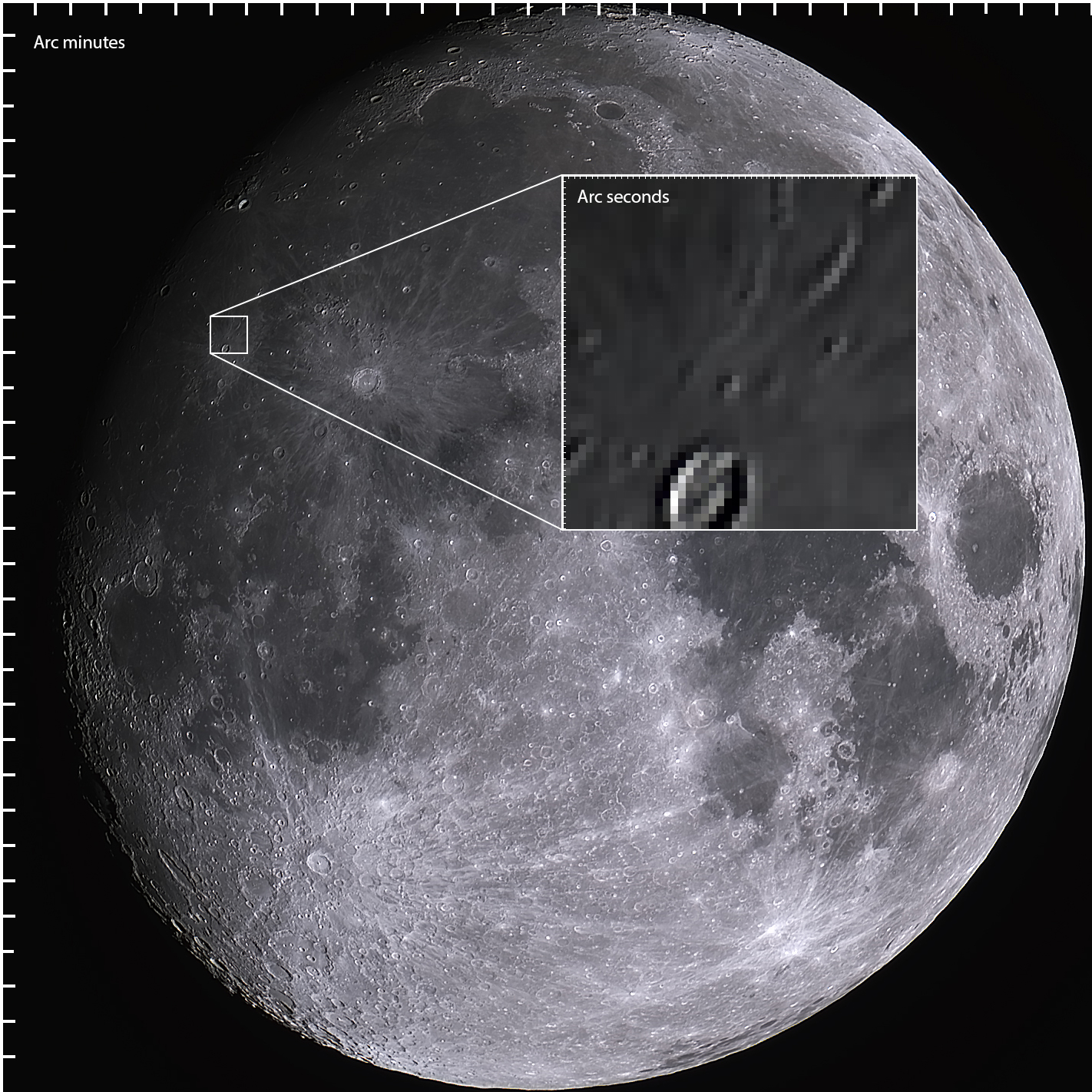
As these units are so commonly used in astrophotography, it's useful to be able to visualise them. To help myself with this, I created the visual aid shown above using my image of the moon. The actual angular size of the full moon varies by a small amount due to the slightly elliptical shape of its orbit. Although the size is normally quoted as 30 arc-minutes, or half a degree, the average is actually about 31, so that's the scale I decided to use. It's important to note that the moon isn't quite full here, but that's been taken into account.

The scale markers along the borders of the image represent arc-minutes. The zoomed-in portion of the image is approximately one square arc-minute, and is labelled with its own scale in arc-seconds. It's interesting to note that the pixels in the image are roughly one arc-second in size, which is a sensible pixel scale for astrophotography. This is again due to the upper limits on useful resolution imposed by atmospheric seeing conditions, and the resulting fact that most telescopes are designed for an image scale somewhere near this range.

When an imaging setup's pixel scale is too small or large, it's known as undersampling and oversampling. If the pixels are too large (for example 5 arc-seconds per pixel under 1 arc-second of seeing), resolution is lost because the pixels can't effectively capture all the available detail. This is undersampling. If the pixels are too small (for example 0.2 arc-seconds per pixel under 1 arc-second of seeing), pixel resolution is wasted because the observable detail is limited by the seeing. This is oversampling. Based on this, it's fair to say my moon image is slightly undersampled.

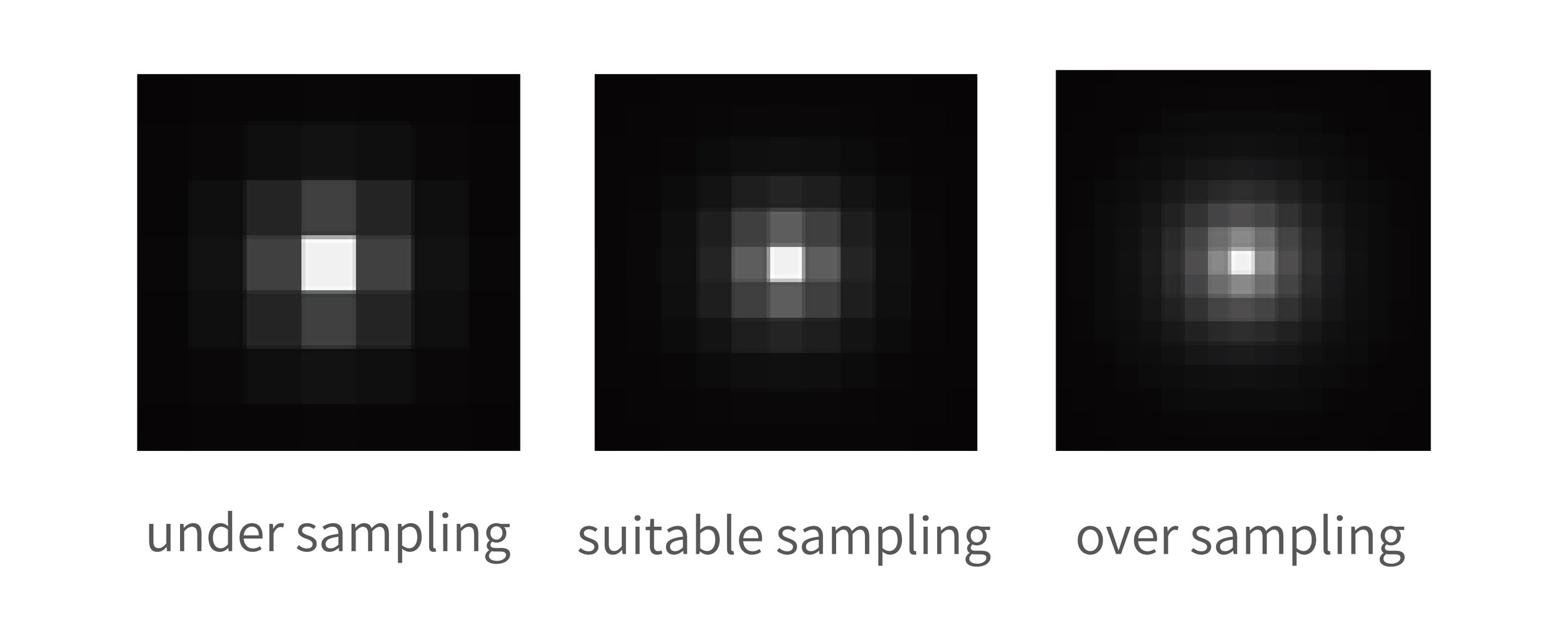
With undersampling, you're obviously just losing detail, and ending up with a blurrier or more pixelated image than necessary. Oversampling is generally not as bad, although neither are ideal. Besides simply wasting pixel resolution which could be put to good use, another important downside to oversampling is that it increases noise by spreading the same amount of signal over a greater number of pixels. As each pixel has some fixed amount of inherent noise, the total noise is more pronounced relative to the signal. There are also small borders between each pixel on the sensor, although in modern designs these are small enough to be disregarded.